FinSight: Leakage-safe financial forecasting
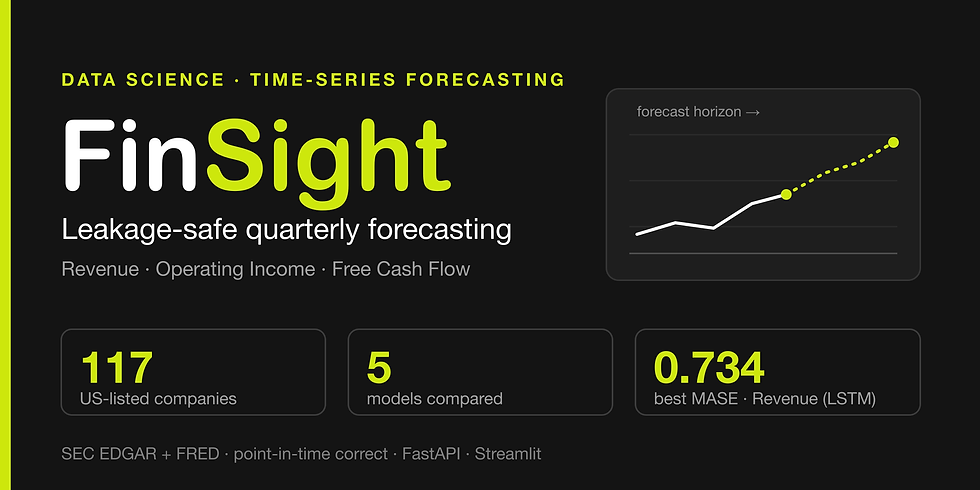
Leakage-safe forecasting of next-quarter Revenue, Operating Income, and Free Cash Flow for 117 US-listed companies — point-in-time SEC EDGAR + FRED data, five models compared, best served per target.

Project Snapshot
Scale / Complexity | Core Technique | Engineering Challenge | Differentiator |
117 companies, 13 years, 5 models | Differenced-target forecasting | Point-in-time data leakage | Honest negative results |
Key Insight
The hardest part of forecasting financials was never the model. It was that the number you want to predict keeps moving: restated after filing, tagged differently across companies, and living on a scale gradient-boosted trees cannot extrapolate across. Every architectural choice traces back to making that target honest before a model ever sees it.
Architecture Diagram

Mermaid source for this diagram
flowchart LR
    subgraph Sources
        SEC[SEC EDGAR<br/>XBRL filings]
        FRED[FRED<br/>macro indicators]
    end
    subgraph Pipeline["Data pipeline"]
        RAW[Raw cache] --> CLEAN[Clean + point-in-time merge] --> FEAT[Feature engineering] --> PANEL[(features.parquet)]
    end
    subgraph Modeling["Five compared models"]
        BASE[Seasonal-naive + Prophet]
        TREES[LightGBM + XGBoost]
        LSTM_[LSTM]
        EVAL[Leaderboard + SHAP]
    end
    subgraph Serving
        TRAIN[Fit + persist] --> MODELS[(production models)] --> API[FastAPI] --> DASH[Streamlit dashboard]
    end
    SEC --> RAW
    FRED --> RAW
    PANEL --> BASE & TREES & LSTM_ --> EVAL
    PANEL --> TRAIN
    PANEL -. historicals .-> DASH
    EVAL -. leaderboard + SHAP .-> DASH
The Problem
Every finance team runs the same exercise before a planning cycle: given everything reported so far, what does next quarter look like? Revenue, operating income, and free cash flow drive budgets, hiring, and guidance. The question sounds like a clean supervised-learning problem: assemble historical financials, add macroeconomic context, train a model to predict the next value.
It is difficult for a reason that has nothing to do with model choice. The inputs come from SEC filings, and SEC filings are not a stable ground truth. A company can restate a quarter months after reporting it (for discontinued operations, an accounting-standard change, or a correction), and the public XBRL data (XBRL is the SEC's machine-readable tagged-filing format) only ever exposes the latest revision. This is not hypothetical: Procter & Gamble's FY2015 operating income was restated after it was first filed, so today's XBRL facts show only the revised figure, the precise leak the project's reconciliation check later catches (see Challenges & Debugging). Two companies reporting the identical economic event can tag it under different XBRL concepts, and the same company can change its tagging when a standard changes (revenue recognition shifted industry-wide with ASC 606 in 2018). Macroeconomic series have the same problem in a different costume: GDP and CPI are revised repeatedly, so the value you read today for 2015 is not the value anyone could have known in 2015.
Anyone can experience this, and most forecasting notebooks do without noticing. They pull "the" revenue number for a period, merge in "the" GDP figure, and train a model on data that silently contains information from the future. The model looks good in backtests precisely because it was allowed to cheat.
Common approaches are insufficient not because the algorithms are weak but because the framing is wrong. The visible problem, "predict next quarter," assumes the target is a fixed, knowable quantity. It is not. The target is a moving object, and the moment you try to pin it down, a hidden constraint surfaces: everything the model learns from must be reconstructed as it was known at the time, and the quantity itself must be reshaped into something a model can actually learn.
Requirements & Constraints
Functional Requirements
Forecast next-quarter Revenue, Operating Income, and Free Cash Flow, one quarter ahead, for a universe of US-listed companies.
Build the dataset from scratch from public sources (SEC EDGAR, FRED), with no pre-packaged datasets.
Compare multiple forecasting approaches under one fair protocol and explain the winner.
Serve forecasts behind an API and an interactive dashboard.
Non-Functional Requirements
No lookahead leakage anywhere in the pipeline: every feature value must be reconstructable as of the filing date it belongs to.
Reproducible from raw ingestion to served model.
Explainable: each feature, transform, model, and metric exists for a stated, defensible reason.
Comparable: every model scored on the same quantity, at the same company-quarters.
Hidden Constraints
Two production realities shaped the architecture more than any modeling choice:
The target is restated and inconsistently tagged. The number to predict is not fixed history; it is history as it was known at a moment. Getting that wrong leaks the future backward.
Gradient-boosted trees cannot extrapolate. A tree leaf predicts the mean of its training targets, so its output is bounded by the range it saw. Train on 2012–2020 and a company that grows past its historical range by 2024 gets clipped at the maximum leaf value. The most obvious target, the revenue level, is the one target a tree structurally cannot forecast for a growing company.
The rest of the system is the story of designing around these two.
High-Level System Design
The pipeline moves in one direction and stores its work in layers, each auditable against the one before it.
Ingestion pulls raw API payloads from SEC EDGAR and FRED to disk, unchanged. This immutable raw layer means every downstream number can be traced back to an exact filing.
Normalization turns filings into a tidy fact table (one row per reported financial fact, carrying its filing date and accession number), then pivots that into an analysis panel of one row per company-quarter. This is where the leakage defenses live: the as-originally-filed value wins when a period appears more than once, and macro indicators are joined at each filing's point-in-time vintage rather than their latest revision.
Feature engineering builds lags, rolling statistics, growth rates, financial ratios, and macro deltas on top of the panel (every feature gated so it is computable as of the row's filing date) and, critically, transforms each target from a level into a one-step-ahead change.
Modeling trains five approaches on that frame under a single rolling-origin backtest, scores them all on reconstructed levels, and explains the interpretable winner with SHAP (Shapley-value feature attributions).
Serving fits the winning model per target on the full history, persists it, and exposes it through a FastAPI service. A Streamlit dashboard sits on top as a pure client of that API and the pre-computed artifacts.
The direction of flow matters: nothing downstream can reach back and change what an earlier layer recorded, which is exactly the property a leakage-sensitive system needs.

Engineering Decisions
Decision 1: Model a differenced change, not the level
Context: The forecast targets are levels: dollars of revenue, operating income, cash flow. The obvious modeling target is that same level. But two of the five models are gradient-boosted trees, and trees cannot extrapolate beyond their training range. Under a chronological 2020 split, any company that grows past its historical ceiling in the test years would have its forecast clipped.
Alternatives Considered.
Option | Advantages | Disadvantages |
Raw levels | Simplest; directly the reported quantity | Cross-company scale dominates; tree learns company size, not dynamics |
Log / asinh levels | Compresses scale across the universe | Keeps the extrapolation ceiling: a compressed level is still a level |
Growth rate y_{t+1}/y_t − 1 | Stationary, scale-free | Divides by a near-zero base for thin operating income and free cash flow |
Margins (revenue growth + margins) | Economically interpretable | Errors compound when reconstructing a level from two separately predicted quantities |
Differenced transform | Bounded, roughly stationary, stays inside the training range | Reconstruction step; asinh scale regimes (see Limitations) |
Final Decision: Predict a one-step-ahead differenced transform: log-growth for Revenue (strictly positive), and an asinh-delta (asinh is the inverse hyperbolic sine, defined for negatives) for Operating Income and Free Cash Flow (both cross zero, where log is undefined). The model forecasts a change; levels are reconstructed by adding the predicted delta to the known current value and inverting the transform. Differencing turns the target into a bounded, roughly stationary quantity that stays inside the training range, and it sidesteps a second tree limitation: a tree cannot learn "input plus delta" as arithmetic, so handing it the delta directly removes a burden it would otherwise have to memorize through splits.
Engineering Principle: Model the transform your estimator can actually learn, then reconstruct the quantity you report, and don't force the estimator to predict a quantity its structure forbids.

Decision 2: Keep the as-originally-filed value, and pull macro data point-in-time
Context: A period can appear in the data more than once: once as originally filed, again after a restatement. Macro series are revised continuously. Using the latest value for either leaks information no one had at the time.
Final Decision: When a fiscal period appears more than once, the earliest filing wins, the number as it was originally public. Heavily revised macro series (GDP, CPI) are pulled through FRED's point-in-time archive (ALFRED), aligned to each filing's date; unrevised market series use latest values because they are never revised. A permanent reconciliation check runs on every ingestion, comparing the sum of derived quarters against the reported annual total, so this discipline is verified continuously rather than assumed.
Engineering Principle: In any time-series system, "the value of X" is incomplete: the question is "the value of X as known when?" Answer that at ingestion, or leak the future everywhere downstream.

Decision 3: Derive operating income from totals, never from a component sum
Context: Many companies (pharma, financials) never tag a clean OperatingIncomeLoss concept. Dropping them would bias the universe toward one shape of income statement. So operating income has to be derived when untagged. The tempting derivation is a component sum: revenue minus cost of goods minus SG&A minus R&D.
Final Decision: Derive from income-statement totals (GrossProfit − OperatingExpenses, else Revenues − CostsAndExpenses), not from a component sum. Validated against companies that do tag operating income, the total-based derivation reproduced the tagged value with a 0.00% median error. The component sum disagreed with issuers' own reported operating income by up to ~42% (Coca-Cola), because it silently omits "other operating" charges like impairments and restructuring. That is a systematic bias, not noise. Every derived row is flagged so tagged and derived values stay separable in later error analysis.
Engineering Principle: When you reconstruct a reported figure, reconstruct it from the same level of aggregation the reporter used. Rebuilding a subtotal from components you can enumerate omits the ones you can't.
Decision 4: Score every model in level space, under one shared mask
Context: The five models live in different spaces. Prophet forecasts levels directly; the trees and the LSTM predict a differenced transform. A level MAE and a delta MAE are not comparable numbers.
Final Decision: No model is ever scored in its own native space. Every prediction is reconstructed to a level and scored there, at the identical set of company-quarters, using per-company MASE (mean absolute scaled error) against a seasonal-naive (four-quarters-prior) benchmark. The denominator is each company's seasonal-naive error on its training window, so a MASE below 1.0 beats that in-sample naive; on the harder evaluation window the naive's own realized MASE sits higher (1.326 / 1.772 / 1.551; see Results), and a model beats the benchmark by scoring below its target's realized naive line. A quarter enters the scored set only if the actual, the baseline, and every model's prediction are all finite, and equal support is asserted. No model is ever quietly scored on fewer points than another.
Engineering Principle: A leaderboard is only meaningful if every row was measured on the same quantity, at the same points. Enforce that as an assertion, not a convention.

Implementation Highlights
Adjacency by time, not by row order: Lag and rolling features derive "the previous quarter" from actual period-end gaps via an integer quarter ordinal, never from row position. A window that would cross a missing quarter emits a null rather than silently pairing two non-consecutive quarters, the kind of bug that never throws an error and quietly corrupts every downstream feature.
Discrete quarters from annual filings: Companies file no standalone Q4 report, and many report cash-flow figures year-to-date. Q4 is derived as the annual figure minus the first three quarters, and YTD flows are differenced into discrete quarters, so every row is a true single-quarter observation.
Per-target inclusion, not per-company: A company can have clean revenue history but unreliable free-cash-flow coverage. Rather than dropping the whole company, inclusion is decided per (company, target): failing one target masks only that target's rows. The universe stays as large as the data honestly supports.
One test module per phase, each runnable standalone: The leakage tests are pure pandas (they assert that every training row's label quarter ended before its origin, that preprocessing statistics use only pre-anchor data) and run without any of the model libraries installed, so the most important invariant in the project is the cheapest thing to check.
Challenges & Debugging
Challenge: A model process that died with no error at all
Investigation: The training process, which fits both LightGBM and an LSTM, sometimes exited with a bare SIGSEGV (exit 139) with no traceback, and under buffered output, no message whatsoever. Other times it produced OMP: Error #179: Function pthread_mutex_init failed. It looked like an infrastructure problem.
Root Cause: LightGBM and PyTorch each ship their own OpenMP runtime. Once torch is imported, LightGBM's first fit or predict (the call that creates its thread pool) kills the process. Measurement made it precise: LightGBM-then-torch succeeds; torch-then-LightGBM fails; and a bare import torch with no torch execution at all is already enough to poison the later LightGBM call. The two standard environment-variable workarounds (KMP_DUPLICATE_LIB_OK, OMP_NUM_THREADS=1) were both tested and do not fix it.
Resolution: The fix is ordering, enforced in two places: the training routine fits all LightGBM targets before any LSTM, and the serving loader warms the LightGBM booster with a dummy predict (constructing the booster is not enough; the warm-up is what claims the runtime) before torch is imported for the LSTM. Both sites carry a load-bearing comment, because the failure looks exactly like something a future cleanup would "simplify" by reordering.
Lesson: A silent, order-dependent failure has to be documented at the site where someone would otherwise break it, and the workarounds you rejected have to be recorded too, otherwise the next person repeats the same experiment.

Challenge: Quarters that didn't add up to the annual
Investigation: The permanent reconciliation check flagged Procter & Gamble's FY2015: the four as-originally-filed quarters summed to $10,952M, 7.11% off the original filed annual operating income. That gap is large enough to look like a parsing bug.
Root Cause: It was not a bug. That same quarterly sum lands within 0.9% of P&G's later-restated annual figure. The quarters disagreed with the original annual because the annual was itself restated after the fact, and the pipeline had correctly kept the figures as they were public at the time.
Resolution: Nothing to fix: the reconciliation check had done its job, distinguishing a data-quality problem from correct point-in-time behavior. A pipeline that pulled "the" annual figure from today's XBRL facts would have silently leaked that restatement backward into 2015.
Lesson: A discrepancy is not automatically an error. A good reconciliation check doesn't just catch bugs; it produces positive evidence that a correctness property is holding.
Results & Evaluation
Five models, one shared scored point set per target, per-company MASE. The MASE denominator is each company's seasonal-naive (four-quarters-prior) error on its training window, so the bar to clear is the naive's own realized MASE on the evaluation window: 1.326 for Revenue, 1.772 for Operating Income, 1.551 for Free Cash Flow. A model beats the benchmark by scoring below its target's naive line, not below a flat 1.0:
Target | Winner | MASE | Served in production |
Revenue | LSTM | 0.734 | LSTM: strongest of four sub-1.0 models on Revenue |
Operating Income | LSTM ≈ LightGBM (statistical tie) | 1.511 / 1.516 | LightGBM: tie broken on explainability |
Free Cash Flow | Seasonal-naive (t−4) | 1.551 | Seasonal-naive: unbeaten by every learned model |
Full five-model leaderboard: every model reconstructed to level space and scored on the identical company-quarters per target (served model in bold; n = scored companies / points):
Target (n companies / points) | Model | MASE |
Revenue (110 / 880) | LSTM | 0.734 |
Prophet | 0.890 | |
LightGBM | 0.917 | |
XGBoost | 0.918 | |
Seasonal-naive (t−4) | 1.326 | |
Operating Income (99 / 792) | LSTM | 1.511 |
LightGBM | 1.516 | |
XGBoost | 1.549 | |
Seasonal-naive (t−4) | 1.772 | |
Prophet | 1.874 | |
Free Cash Flow (106 / 844) | Seasonal-naive (t−4) | 1.551 |
Prophet | 1.581 | |
LightGBM | 1.936 | |
XGBoost | 1.975 | |
LSTM | 5.156 |
Source: reports/phase11_leaderboard.csv. Supporting figures: leaderboard, rolling-origin trajectories (a win driven by one anomalous quarter would show here), and residual analysis:


Revenue is genuinely forecastable: All four learned models clear the seasonal-naive on Revenue: Prophet (0.890), LightGBM (0.917), and XGBoost (0.918) all land under a MASE of 1.0, but the LSTM leads the field decisively at 0.734. It is the only model that consumes the ordered sequence rather than a flat feature vector, and its margin over the trees, which see the identical features flattened, isolates the value of temporal structure. The edge is broad, not an artifact of averaging: per company, the LSTM beats the seasonal-naive on 80 of 110 companies (72.7%). A decisive win, not a solitary one.
Operating Income is a statistical tie: LightGBM (1.516) and the LSTM (1.511) are separated by less than a third of a percent, a gap well inside the noise of a single-seed, 99-company (792-point) averaged metric, and not a meaningful ordering. Both clear the naive's 1.772 despite sitting above 1.0, beating the benchmark on the evaluation window even though neither reaches the stricter sub-1.0 mark. So the winner is not read off the third decimal; the tie is broken on explainability instead: SHAP explains the LightGBM model exactly via a tree explainer, so the interpretable model is served over the indistinguishable one that cannot be.
Free Cash Flow is an honest negative result: No learned model (not the LSTM, not either tree, not Prophet) beat simply predicting the value four quarters ago. So the seasonal-naive baseline is what gets served for this target, and the API and dashboard say so explicitly, rather than shipping a worse learned model to look more sophisticated.
Explainability: SHAP on the production LightGBM model shows each target's strongest driver is its own autoregressive quarter-over-quarter change, exactly what you'd expect from a one-step-ahead differenced forecaster, which is a useful sanity check that the model learned dynamics rather than an artifact.

Limitations
Survivorship bias. The 117-company universe is drawn from present-day listings, so firms that delisted, went bankrupt, or were acquired since 2012 are absent. Results are mildly optimistic relative to a true point-in-time universe. Accepted and documented for v1 rather than reconstructing historical index membership.
asinh scale regimes. The asinh-delta target handles values that cross zero, but asinh is near-linear near the origin and log-like for large magnitudes, so companies spanning single-digit-million to tens-of-billions of free cash flow sit in different regimes of the same transform. Fixing units at millions mitigates this but does not remove it.
One quarter ahead only. The horizon is a single quarter; multi-quarter forecasting would compound reconstruction error and needs its own evaluation.
Free Cash Flow remains unbeaten by learning. The negative result is honest, not solved: the naive baseline is genuinely the best available forecast for this target here.
No uncertainty quantification on the leaderboard. The per-company MASE figures are single-run point estimates under a fixed seed: reproducible, but one draw. The LSTM is stochastic; neither its seed-variance nor forecast intervals are quantified. Close results should therefore be read as indistinguishable rather than ordered (Operating Income is the clear case), and even Revenue's sub-1.0 edge is one seed's result, not a distribution. Confidence intervals are a deferred v1-stretch item, not a claim made here.
Production operations are out of v1 scope. Serving stops at fitting the winning model per target, persisting it, and exposing it behind FastAPI. Retraining cadence and triggers, drift detection, model versioning and rollback, and monitoring/alerting are deliberately deferred: v1 demonstrates a correct, reproducible build, not an operated service. Consistent with the out-of-scope boundary (no orchestration, no cloud deployment).
Batch scale by design. The 117-company universe is processed as a batch, with the analysis panel held in memory as a single parquet frame. A materially larger universe or a higher refresh frequency would pressure that in-memory panel and the ingestion pass first; distributed processing, streaming, and orchestration (Spark, Kafka, Airflow, Kubernetes, cloud) are explicitly out of scope for v1.
Lessons Learned
Lesson 1: Reshape the target to fit the estimator. The differenced-target decision generalizes to any bounded-output estimator: when the quantity you report lies outside what your model can structurally produce, change what you predict before you change how hard you try to predict it, then reconstruct the reported quantity afterward.
Lesson 2: "The value of X" is a question about time. Every leakage defense in this project reduces to answering as known when? through as-originally-filed values, point-in-time macro vintages, and features gated to their filing date. In time series, a value without a knowledge date is a leak waiting to happen.
Lesson 3: A negative result reported honestly is worth more than a positive result dressed up. Serving the naive baseline for free cash flow, and saying so, is more credible than serving a learned model that quietly does worse. The willingness to report the failure is itself the evidence of rigor.
Lesson 4: Document constraints where they'll be violated. The OpenMP ordering isn't obvious from reading either library, and its failure is silent. Writing it at both enforcement sites (plus the rejected workarounds) is what keeps a future cleanup from reintroducing a segfault with no traceback.
Future Improvements
Confidence intervals on forecasts, plus seed-variance on the leaderboard (currently single-seed point estimates only)
Multi-quarter-ahead forecasting
Scenario analysis (sensitivity to macroeconomic shocks)
Reconstructing as-of-date index membership to remove survivorship bias
Production operations: retraining cadence and drift-triggered refresh (currently fit-once and persisted), model versioning and rollback, and serving monitoring
Experiment tracking (MLflow) and container packaging for reproducibility
Technology Stack
Category | Technologies |
Data | SEC EDGAR (XBRL), FRED / ALFRED (point-in-time) |
ML | scikit-learn, LightGBM, XGBoost, Prophet, PyTorch, SHAP |
Backend | FastAPI |
Dashboard | Streamlit, Plotly |
Tooling | Python 3.12, uv, Ruff, pytest |
The Principle Worth Keeping
A forecasting system is only as honest as the target it trains on. Most of the engineering in FinSight went not into choosing an algorithm but into making the target trustworthy before any algorithm saw it: reconstructing values as they were known at the time, reshaping levels into changes a model can actually learn, and reporting a benchmark-beating baseline as the winner when it genuinely was. Design around the constraints that stay invisible during development and dominate in production, and the model becomes the easy part.